How to Build a Binary Search Tree in JavaScript

Data structures are all around us, but you often don’t notice them unless you’re a software engineer or data scientist. Data structures are fundamental to computer programming and working with data in general. Having a strong grasp of data structures and their inner workings is critical to succeeding in these fields, so taking the time to learn about them in detail can be very rewarding.

Binary Search Tree (BST)

A binary search tree is a combination of a tree data structure and the binary search algorithm. The data is rigidly organized in the tree structure in a way that is conducive for a binary search. While there are limitations associated with using this structure, there are certain scenarios where a BST is the best choice for the task at hand. We’ll dive into that a bit later.

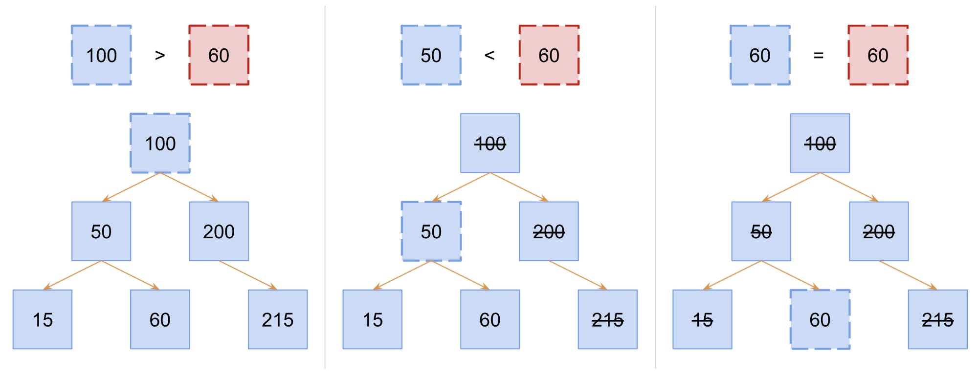
First, we need to build a mental model. It’s important to have a fully-formed mental model before you dig into efficiency or code. So let’s take a look at a visualization of how search works in a BST.

The illustration shows how the algorithm would search for the value 60 in a BST. The value comparison at each iteration of the search is shown at the top. The BST illustration at the bottom is updated for each iteration to show the current node for comparison (shown with a dotted border) and the nodes that have been eliminated from consideration (shown with strikethrough text).

Binary search is a little more elegant than your typical search because it utilizes the data organization to its advantage. Like searching for a word in a dictionary or glossary, you wouldn’t just start at the first page and turn every single page until you found your word. Instead, you might open the book to roughly where you think the word might be alphabetical, compare your word to a word on the page to see if your word comes before or after, and then use that knowledge to jump to a different page that should be closer to your target word. Once you get to a page that is pretty close, you might start turning individual pages so that you don’t overshoot your page estimates.

The data is organized where the left child value is always less than the parent and the right child value is always greater than the parent.

A binary search tree works in the same way. On each iteration, you compare your values, and if they’re not equal, you eliminate the half of the tree where your target value could not exist. This is all possible because the data is organized where the left child value is always less than the parent and the right child value is always greater than the parent. Thus, if you know your value is greater than the value at the current node, you can eliminate the left child and all of its descendants from consideration.

As I’ve alluded to previously, this design has some useful efficiency characteristics that we’ll discuss next.

Efficiency

Consuming data structures without understanding their efficiencies is kind of like the average person using kitchen knives. You can slice an apple with a steak knife, but some knives are much better suited for the job. To know which knife to use, you need to know what each knife is designed to do. Similarly, to know which data structure to use you inherently need to understand their efficiencies.

To understand the efficiencies of a data structure, you must know the language in which efficiencies are communicated. That language is called Big O notation and it’s commonly used in engineering, data science, and mathematics. Additionally, a single data structure’s efficiencies aren’t particularly useful in isolation. They only truly become useful when you compare them to each other. As you’re learning about data structures and their efficiencies, you can reference this cheatsheet that I’ve found helpful in the past.

Now when we discuss data structure efficiency, we usually only discuss them in terms of time complexity. This is because most data structures have linear space complexity (i.e. O(n)) so it would be fairly trivial to compare them. Also, we often will only be interested in the worst-case scenarios because typical scenarios won’t usually overstress our machine resources.

However, in the case where we need to search for items rather often, a BST is particularly optimized to do exactly that. In particular, the BST has O(log(n)) time complexity for the average case. That means that sometimes you might search for an element that is at the very end of your tree and your time complexity for a single search would be O(n), but because half of your tree elements are eliminated on each iteration of the search, your typical time complexity will be less than linear.

Now there is another data structure that has even better search time complexity, and that is the hash table. However, the binary search tree is better suited for scenarios where you’re data’s relations with its neighboring data matter. If you need to get adjacent data points or a data range, it might be more optimal to use a BST rather than a hash table.

Implementation in JavaScript

Generally speaking, to implement a binary search tree you’re going to need to implement a node that is going to represent each element in your tree. Nodes in a BST need to support a value, left, and right properties. The left and right properties are pointers that point to the child nodes that adhere to the rigid structure of the BST. Specifically, the left node must have a value that is less than its parent, and the right node’s value must be greater than its parent’s value. Below is a class implementation of a Node.

This class is pretty straightforward. You must instantiate your class with a value, and you can optionally designate left and right nodes initially as well.

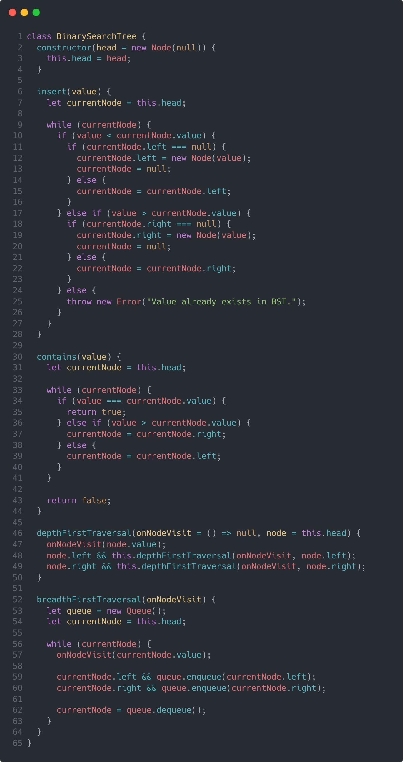
Now that we have our Node class, we can use it in our BinarySearchTree class to build out our functionality. Our BinarySearchTree class will have an insert method to add a node to the tree and a contains method to check whether a BST currently has that value already. Additionally, I’ll show you how to implement a depth-first traversal and a breadth-first traversal through this BST. While not all necessary for this exercise, it might be helpful to see how these traversals work for your overall understanding of how binary search trees work.

Let’s check out the code:

Now, let’s break down each part of this class in more detail.

The Constructor

The BinarySearchTree class itself mostly just acts as a housing for the head node. We need to keep a reference to our head because every other node in our tree originates from that node. So if we want to insert a new node into the tree, we have to start from the head because it dictates where all other nodes are placed. I’ve also opted to provide this value with a default assignment of an empty Node instance. That way I can rely on there being a head node present and not have to code defensively around that.

The insert() Method

The insert method is a critical method for any binary search tree because of the strict ordering each node has to adhere to. Remember, the left node must have a value less than its parent, and the right node’s value must be greater than that of its parent.

As for the algorithm, it’s quite simple. We traverse through the tree using a while loop that runs until we are out of nodes to check. On each iteration, we compare the value to be inserted to the value of the current node we’re on. That tells us which side to continue traversing, the left or the right. Then, if there’s no child node on that side (i.e. left or right are null), we’ll insert a new node with our new value. Otherwise, if there is a child node there, we’ll set that to be our new current node and the loop continues.

The contains() Method

This method checks whether or not the BinarySearchTree instance contains the value parameter provided. The logic here is similar to that of insert(), but a little simpler. We still traverse through the tree using a while loop and compare the target value to the current node value. However, instead of looking for the end of the tree (also known as a “leaf” node) so that we may insert a new node there, we now only need to compare values for equality. We continue the traversal until we find the target value or we run out of nodes.

The depthFirstTraversal() Method

As I mentioned earlier, this method isn’t really necessary, but I find it helpful to compare it to the breadthFirstTraversal() method, so I added it. And since our contains() method already technically does a depth-first traversal, I decided to implement this method using recursion instead of the iterative method I used in contains().

Recursion can be a tricky concept to conceptualize, so if you’re having trouble wrapping your head around it, check out this video that I found very helpful. Otherwise, the method is quite simple and concise. The method accepts two parameters: a callback to be invoked on every iteration and a starting node. The callback has a default assignment that essentially amounts to a “no-op” function, and the starting node defaults to the head node. From there, we simply invoke our callback with the current value passed in and then recursively call our method with the left and right nodes respectively, if they exist.

The breadthFirstTraversal() Method

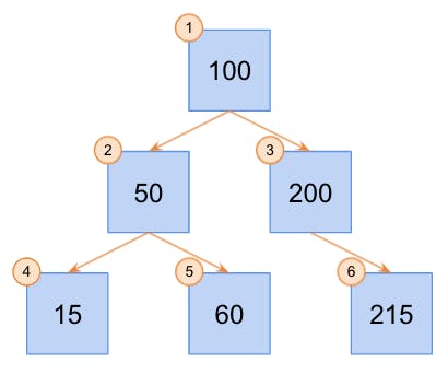
Similarly, I added this method as a little bonus to illustrate how you might traverse a tree using a breadth-first strategy. Breadth-first search is a little less intuitive than depth-first search, but with the proper mental model, the logic is pretty simple. First, let’s illustrate our process.

An illustration of breadth-first search in a binary tree

The above illustration shows how we traverse through each “row” completely before we move on to the next one. Conversely, with depth-first traversal, we iterate through a branch in its entirety before moving on to the next branch.

There are a few different ways to design this algorithm, but the general idea is to traverse through the tree, and along the way, place a reference to each of those nodes in the order that you want them. Then, you can simply iterate through your ordered references. As described above, we completely traverse through each “row” first, then we move on to the next “row”. So, we’ll run through this sub-routine for each “row”. In my solution, we’ll reorder references to each node using a queue, then when we dequeue them, they’ll be removed from the queue in the proper order.

If you’re unfamiliar with the queue data structure, please check out this article I’ve written where I describe them in detail and show you how to build a Queue class in JavaScript.

Conclusion

The binary search tree is a unique data structure that is designed with search efficiency in mind. Hopefully, this article has been useful to you, and if it has, please give me a follow so you’ll be the first to know when I post more content. Thanks!